Chapman Is Not Enough
The Chapman cycle contains O2, O, O3, photons, and a third body M.
It is useful for gas-phase ozone photochemistry, but it is not a good teaching case for rainout.
PROFILE NODE
Using the modern sulfur cycle to understand rainout rates, Henry constants, and the wetdep array.
Student Handout
Lecture 4 used the Chapman cycle to introduce emission and dry deposition.
Wet deposition is different: it is not a useful Chapman-cycle example.
In this lecture, we switch to the modern sulfur cycle, where soluble sulfur species can be removed by cloud water and precipitation.
The goal is to understand how PATMO stores and applies wet deposition rates in the code, and how a species-specific rainout rate becomes a loss term in the model equations.
The PATMO paper by Danielache et al. (2023) describes PATMO as a flexible one-dimensional atmospheric chemistry code. In that framework, atmospheric composition is controlled not only by chemistry and photolysis, but also by boundary and removal processes such as surface emission, dry deposition, wet deposition, condensation, sedimentation, diffusion, and escape.
This lecture focuses on the wet-deposition part of that physical picture and connects it to the actual PATMO code used in the modern sulfur cycle case.
Chapman Is Not Enough
The Chapman cycle contains O2, O, O3, photons, and a third body M.
It is useful for gas-phase ozone photochemistry, but it is not a good teaching case for rainout.
Sulfur Has Soluble Species
The modern sulfur cycle includes species such as SO2, SO4, H2S, OCS, and CS2.
Some of these species can interact with water and be removed by wet deposition.
| File | What students should notice |
|---|---|
src_f90/patmo_parameters.f90 |
wetdep(cellsNumber, chemSpeciesNumber) stores wet-deposition rates for each layer and chemical species. |
src_f90/patmo_ode.f90 |
The ODE system subtracts wetdep(j,i) * n(j,i) from layer j. For layers above the surface, the same amount is added to the layer below. |
tests/modern_sulfur_cycle/test.f90 |
The modern sulfur cycle test initializes wetdep and calls computewetdep(idx, Heff) for selected sulfur species. |
tests/modern_sulfur_cycle/Rainout-SO2.txt |
The generated rainout file lists altitude ZKM and K_RAIN, the first-order wet-deposition rate. |

Rainout-SO2.txt.
The legend identifies K_RAIN as the first-order wet-deposition rate used by wetdep(j,i).
The original PATMO ODE code applies wet deposition like this:
! Wet Deposition
do j = 12, 2, -1
    do i = 1, chemSpeciesNumber
        dn(j,     i) = dn(j,     i) - wetdep(j, i) * n(j, i)
        dn(j - 1, i) = dn(j - 1, i) + wetdep(j, i) * n(j, i)
    end do
end do

do i = 1, chemSpeciesNumber
    dn(1, i) = dn(1, i) - wetdep(1, i) * n(1, i)
end do
In the code, wet deposition is a first-order process. For species i in layer j:
In PATMO notation, \(k_{\mathrm{rain},j,i}\) is stored as wetdep(j,i).
The unit is \(\mathrm{s^{-1}}\). The product wetdep(j,i) * n(j,i)
has units of molecules cm\(^{-3}\) s\(^{-1}\).
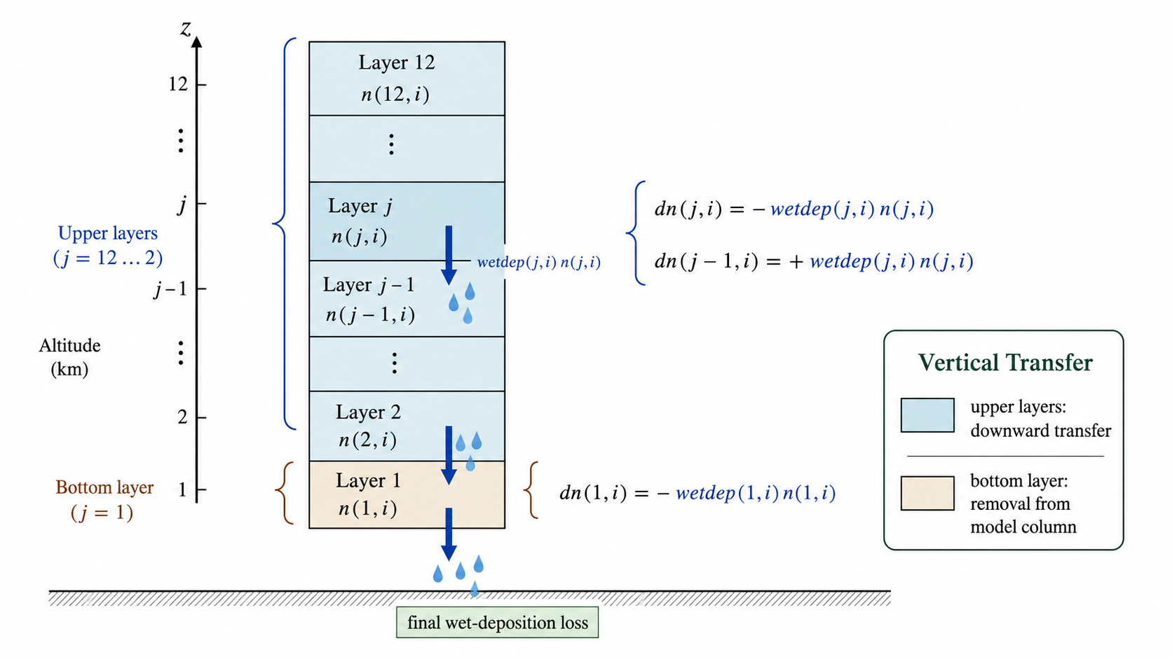
Upper Layers
For j = 12 down to 2, PATMO subtracts wetdep(j,i) * n(j,i)
from the current layer and adds the same amount to the layer below.
This represents rainout moving material downward through the column.
Bottom Layer
For j = 1, there is no lower atmospheric layer.
The code subtracts wetdep(1,i) * n(1,i) from the model column, so the bottom-layer term is the final removal by wet deposition.
Vertical Transfer
PATMO does not only delete material from every layer.
For layers j = 12 down to 2, material removed from layer j is added to layer j - 1.
In the bottom layer, wet deposition is a true loss from the model column.
In tests/modern_sulfur_cycle/test.f90, PATMO computes rainout for selected sulfur species by passing an effective Henry constant:
wetdep(:,:) = 0d0

call computewetdep(1,  2.0d-2)  ! OCS
call computewetdep(11, 5.0d-2)  ! CS2
call computewetdep(28, 1.0d-1)  ! H2S
call computewetdep(18, 4.0d3)   ! SO2
call computewetdep(19, 5.0d14)  ! SO4
Species Index
The first argument is the PATMO species index.
For example, 18 is used for SO2 in this generated mechanism.
Heff
The second argument is the effective Henry constant used by computewetdep.
Larger values generally mean stronger coupling to water and faster rainout.
This calculation answers one question:
how fast should species i be removed by rainout in layer j?
The answer is a first-order rate constant called K_RAIN.
Read the calculation in three steps: estimate contact with water, correct for precipitation timing, then convert the result into a first-order loss rate.
1. Water Available
WH2O represents the layer-dependent water removal term used by the rainout calculation.
More available liquid-water removal generally gives stronger wet deposition.
2. Solubility
Heff is the effective Henry constant for the species.
A more soluble species is more easily transferred into water and can rain out faster.
3. Timing
gamma is a precipitation/non-precipitation time factor, and fz is an altitude-dependent factor.
Together they prevent the simple removal frequency from being used too directly.
First, computewetdep estimates a raw layer-dependent removal frequency \(r_{j,i}\).
This is not the final rainout rate yet. It is an intermediate estimate of how quickly species i
can be transferred into water in layer j:
In this expression, \(W_{\mathrm{H2O},j}\) comes from the vertical water profile, \(H_{\mathrm{eff},i}\) is species-specific, \(T_j\) is the layer temperature, and \(R\) is the gas constant in the unit system used by the code.
Second, the code computes a correction factor \(Q_j\). This correction accounts for the fact that rainout is not simply continuous removal at the raw frequency \(r_{j,i}\):
\[ Q_j = 1 - f_z + \frac{f_z}{\gamma_j r_{j,i}} \left(1 - e^{-r_{j,i}\gamma_j}\right) \]Third, the corrected first-order rainout rate is calculated as:
\[ K_{\mathrm{RAIN},j,i} = \frac{1 - e^{-r_{j,i}\gamma_j}}{\gamma_j Q_j} \]
This K_RAIN value is what becomes wetdep(j,i) in the ODE system.
Once it is stored there, PATMO uses it exactly like any other first-order sink:
K_RAIN * [species].
Reading Shortcut
You do not need to memorize every term in the rainout formula.
For this lecture, remember the workflow:
choose a species, provide Heff, let computewetdep calculate K_RAIN(z),
and use K_RAIN as the first-order wet-deposition rate in each layer.
In the modern sulfur cycle test, wet deposition is assigned directly in
tests/modern_sulfur_cycle/test.f90. The model first clears all wet-deposition rates,
then assigns rainout to selected sulfur species.
wetdep(:,:) = 0d0

! calculate wet deposition
call computewetdep(1,  2.0d-2)  ! OCS
call computewetdep(11, 5.0d-2)  ! CS2
call computewetdep(28, 1.0d-1)  ! H2S
call computewetdep(18, 4.0d3)   ! SO2
! call computewetdep(26, 5d14)  ! H2SO4
call computewetdep(19, 5d14)    ! SO4

! Turco H2SO4
wetdep(12,26) = 1.77E-06
wetdep(11,26) = 3.54E-06
wetdep(10,26) = 5.31E-06
wetdep(9,26)  = 7.08E-06
wetdep(8,26)  = 8.85E-06
wetdep(7,26)  = 1.06E-05
wetdep(6,26)  = 1.24E-05
wetdep(5,26)  = 1.42E-05
wetdep(4,26)  = 1.59E-05
wetdep(3,26)  = 1.77E-05
wetdep(2,26)  = 1.95E-05
wetdep(1,26) = 2.12E-05| Species | PATMO index | How wet deposition is assigned | What students should notice |
|---|---|---|---|
OCS |
1 |
computewetdep(1, 2.0d-2) |
The second argument is the effective Henry constant used to calculate K_RAIN(z). |
CS2 |
11 |
computewetdep(11, 5.0d-2) |
Less soluble species receive smaller rainout rates than highly soluble sulfur species. |
H2S |
28 |
computewetdep(28, 1.0d-1) |
The species index must match the generated PATMO mechanism. |
SO2 |
18 |
computewetdep(18, 4.0d3) |
This is the example connected to the Rainout-SO2.txt profile shown above. |
SO4 |
19 |
computewetdep(19, 5d14) |
A very large effective Henry constant makes sulfate strongly coupled to wet removal. |
H2SO4 |
26 |
Manual values: wetdep(layer,26) |
The computewetdep call is commented out, so this test prescribes an H2SO4 vertical profile directly. |
Computed Species
For OCS, CS2, H2S, SO2, and SO4, the code supplies
computewetdep with a species index and an effective Henry constant.
PATMO then calculates the layer-dependent wetdep(j,i) profile.
Prescribed H2SO4
For H2SO4, the code uses explicit values from layer 12 to layer 1.
These numbers are already first-order wet-deposition rates in s-1, so they can be placed directly into
wetdep(layer,26).
Model Meaning
Once these lines are executed, each value of wetdep(j,i) is used by the ODE as a first-order term.
For example, the SO2 loss or transfer rate in layer j is
wetdep(j,18) * n(j,18).
1. Choose Species
Start with a sulfur species in the modern sulfur mechanism, such as SO2 or SO4.
2. Find Heff
Find or justify an effective Henry constant for the species. Record the source and units.
3. Compute K_RAIN
Use computewetdep(idx, Heff) or assign wetdep(layer,idx) directly when a prescribed vertical profile is used.
4. Put It In The ODE
Interpret wetdep(j,i) as a first-order rate: K_RAIN * [species].