Dry Deposition
Ozone dry deposition can occur on vegetation, soil, water, snow, building surfaces, and other lower-boundary surfaces. The wheat-canopy paper below is only one literature example for learning how to find a deposition velocity.
PROFILE NODE
Adding emission and dry deposition around the Chapman cycle.
Student Handout
Lecture 2 and Lecture 3 used the Chapman cycle to build a gas-phase reaction network. The cycle itself contains thermal reactions and photochemical reactions:
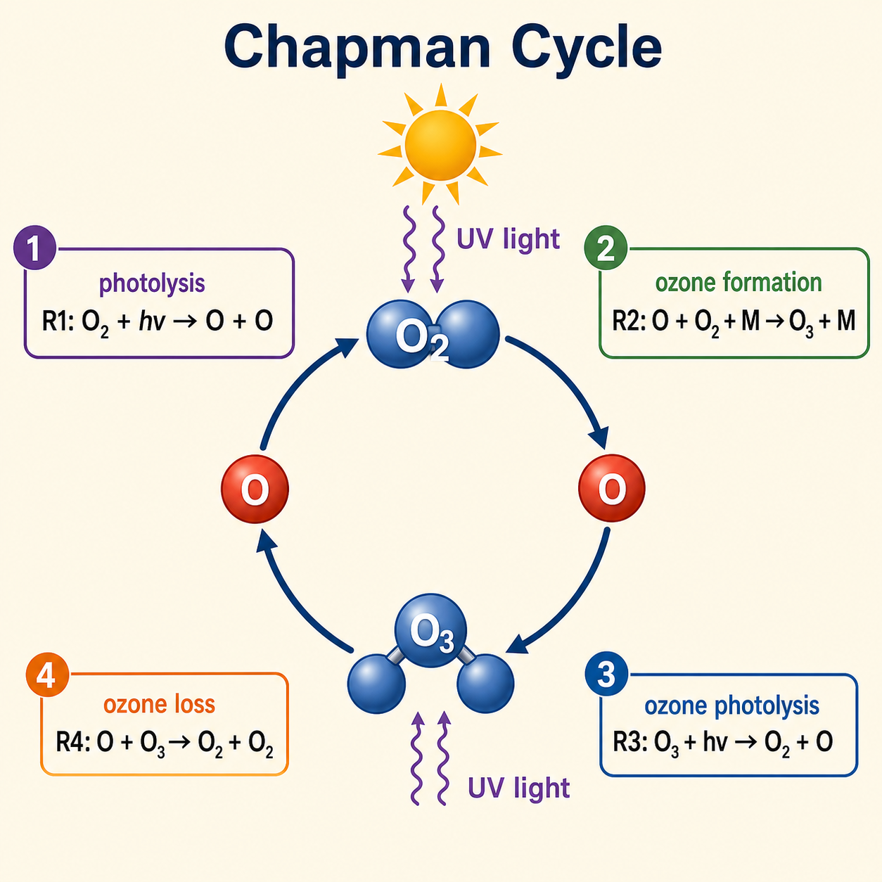
R1: O2 + hv -> O + O
R2: O + O2 + M -> O3 + M
R3: O3 + hv -> O2 + O
R4: O + O3 -> O2 + O2
In this lecture, we keep that same Chapman network and add two processes around it: emission and dry deposition. These are not new Chapman chemical reactions. They are source and sink terms that add or remove species from the model column.
For one species \(i\), the model tendency can be written as:
\[ \frac{dn_i}{dt} = P_i^{\mathrm{chem}} - L_i^{\mathrm{chem}} + S_i^{\mathrm{emission}} - L_i^{\mathrm{dry}} \]The Chapman cycle gives the chemical production and loss terms. Emission adds material. Dry deposition removes material at the lower boundary. In a pure Chapman-only exercise, these two extra terms can be set to zero.
Important Point
Do not write emission or deposition as ordinary gas-phase reactions such as
O3 -> surface inside the Chapman reaction list.
They are physical source and sink processes with their own units and model settings.
Dry Deposition
Ozone dry deposition can occur on vegetation, soil, water, snow, building surfaces, and other lower-boundary surfaces. The wheat-canopy paper below is only one literature example for learning how to find a deposition velocity.
Emission
For a simple classroom demonstration, use a direct artificial O3 emission flux.
This makes the input format and unit conversion easy to see, even though real lower-atmosphere ozone is usually produced photochemically.
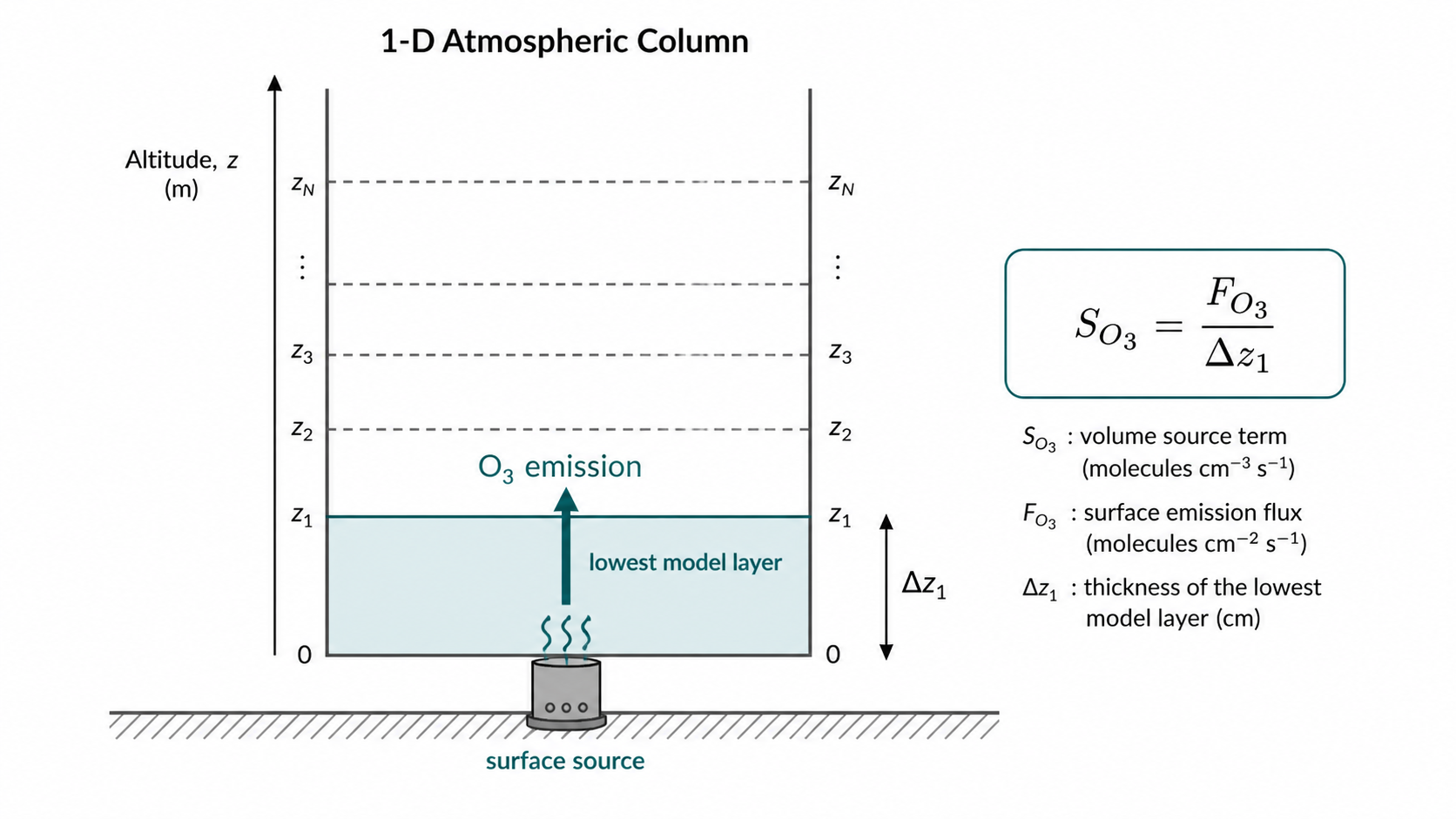
Emission means a species is added to the model from a source. In a one-dimensional column, the most common teaching form is a surface flux into the lowest model layer.
\[ S_i^{\mathrm{emission}} \approx \frac{F_i}{\Delta z_1} \]\(F_i\) is the emission flux, often written in molecules cm\(^{-2}\) s\(^{-1}\). \(\Delta z_1\) is the thickness of the lowest model layer. After division by \(\Delta z_1\), the source term has volume units such as molecules cm\(^{-3}\) s\(^{-1}\).
Chapman Example
For a physically clean Chapman baseline, set direct emissions of O, O2, and O3 to zero.
If the class adds an ozone emission term, treat it as a controlled numerical experiment:
the purpose is to learn how a source term changes the ozone budget, not to claim ozone is normally emitted this way.
In this lecture, use a direct O3 emission only as a training source.
The goal is not to claim that surface ozone is normally emitted this way.
The goal is to show how students can find a reported O3 emission rate in the literature,
convert its units, and place it into the lowest model layer.
A useful example is
Link et al. (2023),
which reports ozone generation from a 222 nm germicidal ultraviolet lamp.
The paper gives an O3 generation rate of 1.22 mg h-1.
Step 1: Search The Literature
Use keywords such as ozone emission rate mg h-1, O3 generation rate UV lamp,
or ozone generator emission rate. Keep papers that report a direct O3 rate with units.
Step 2: Copy The Reported Value
From Link et al. (2023), copy the species, source type, value, and unit:
O3, UV lamp generation, \(R_{\mathrm{mass}} = 1.22\) mg h\(^{-1}\).
Step 3: Choose Model Geometry
The paper reports a total generation rate, not an atmospheric surface flux. For a 1D teaching column, assume a column area \(A = 1\) m\(^2\) and lowest-layer thickness \(\Delta z_1 = 1000\) m.
Step 4: Convert To Model Units
Convert mg h\(^{-1}\) to molecules cm\(^{-2}\) s\(^{-1}\), then divide by \(\Delta z_1\). The final source term should be in molecules cm\(^{-3}\) s\(^{-1}\).
Worked Conversion
First convert the total mass rate to a mass flux over the chosen model column area:
\[ E_{\mathrm{mass}} = \frac{R_{\mathrm{mass}}}{A} = \frac{1.22 \times 10^{-3}\ \mathrm{g\ h^{-1}}}{1\ \mathrm{m^2}} = 1.22 \times 10^{-3}\ \mathrm{g\ m^{-2}\ h^{-1}} \]Then convert the mass flux to a number flux using \(M_{\mathrm{O_3}} = 48.00\) g mol\(^{-1}\):
\[ F_{\mathrm{O_3}} = E_{\mathrm{mass}} \frac{N_A}{M_{\mathrm{O_3}}} \frac{1}{10^4} \frac{1}{3600} \approx 4.25 \times 10^{11} \ \mathrm{molecules\ cm^{-2}\ s^{-1}} \]Finally divide by the layer thickness \(\Delta z_1 = 1000\) m \(= 1.0 \times 10^5\) cm:
\[ S_{\mathrm{O_3}} = \frac{F_{\mathrm{O_3}}}{\Delta z_1} = \frac{4.25 \times 10^{11}}{1.0 \times 10^5} \approx 4.25 \times 10^6 \ \mathrm{molecules\ cm^{-3}\ s^{-1}} \]
This is the value students can place into the O3 source term for the artificial emission demonstration.
If they choose a different paper value, column area, or model-layer thickness, they must redo the conversion.
Teaching Use In This Case
Use this direct O3 emission only to teach how a source term is written in PATMO.
In the physical baseline, the teacher may still set direct O3 emission to zero and then turn on this artificial source as a sensitivity test.
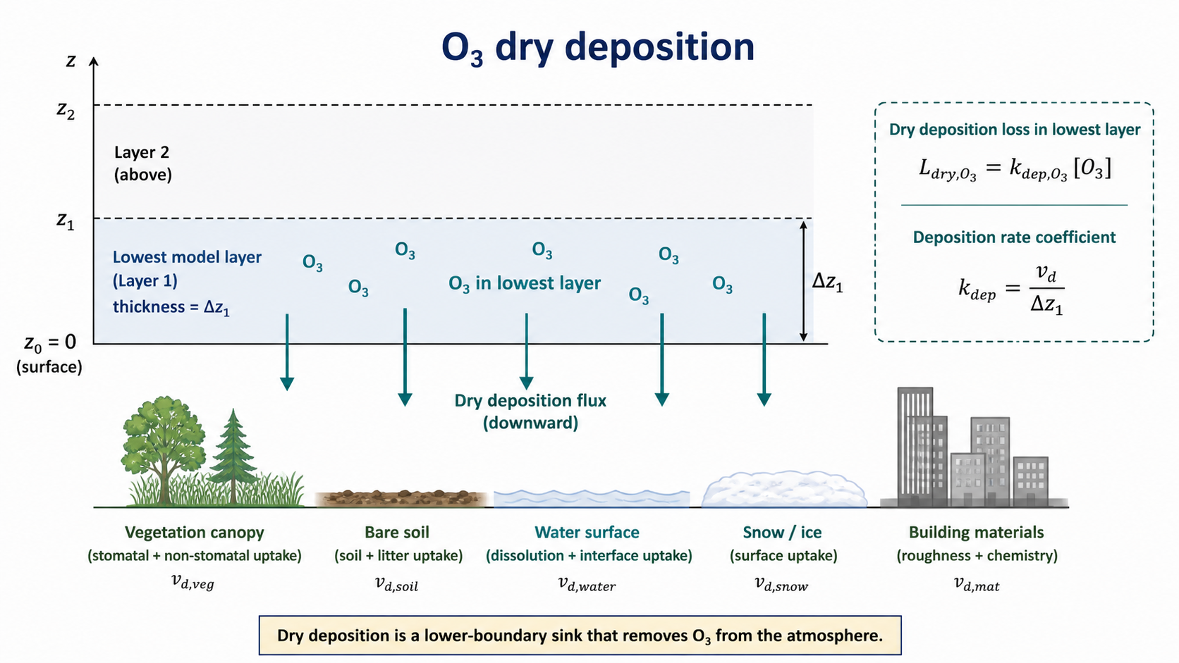
Dry deposition is removal at the lower boundary without precipitation. It is usually written with a deposition velocity \(v_{d,i}\):
\[ F_i^{\mathrm{dry}} = v_{d,i} n_i(z_1) \] \[ L_i^{\mathrm{dry}} \approx \frac{F_i^{\mathrm{dry}}}{\Delta z_1} = \frac{v_{d,i} n_i(z_1)}{\Delta z_1} \]\(n_i(z_1)\) is the species concentration in the lowest layer. \(v_{d,i}\) has units of length per time, such as cm s\(^{-1}\). A larger deposition velocity means faster surface removal.
Chapman Example
Apply dry deposition to O3 as the worked Chapman example.
This creates a surface sink that competes with photolysis and the gas-phase loss reaction
O + O3 -> O2 + O2.
Use vegetation as the example surface and search for a recent paper with these keywords:
ozone dry deposition velocity wheat field, O3 deposition flux vegetation, or
Vd ozone cropland.
A good example is Zhang et al. (2024), which measured ozone deposition over wheat fields in the North China Plain during the 2023 wheat growing season.
Step 1: Identify The Surface
Record the land surface before copying any number. In this paper, the surface is a wheat canopy, not bare soil, open water, or forest.
Step 2: Find The Variable
Search inside the paper for deposition velocity, Vd, and flux.
For PATMO, the number we need for the simple dry-deposition setting is usually a deposition velocity.
Step 3: Copy Units
Zhang et al. report deposition velocity in cm s\(^{-1}\). The reported mean value for the main wheat growing season is \(V_d = 0.29 \pm 0.33\) cm s\(^{-1}\).
Step 4: Keep Context
The same paper reports higher daytime \(V_d\) than nighttime \(V_d\). Do not treat one value as universal: record site, season, vegetation type, method, and whether the value is daytime, nighttime, or all-period average.
Worked Conversion For Model
The reported value \(V_d = 0.29\) cm s\(^{-1}\) is already a deposition velocity. If PATMO asks directly for a dry-deposition velocity, students can enter:
\[ v_{d,\mathrm{O_3}} = 0.29\ \mathrm{cm\ s^{-1}} \]If the model setup needs a lowest-layer first-order loss rate, divide by the lowest-layer thickness. With \(\Delta z_1 = 1000\) m \(= 1.0 \times 10^5\) cm:
\[ k_{\mathrm{dep,O_3}} = \frac{v_{d,\mathrm{O_3}}}{\Delta z_1} = \frac{0.29}{1.0 \times 10^5} \approx 2.9 \times 10^{-6}\ \mathrm{s^{-1}} \]The volume loss term is then this first-order rate multiplied by the lowest-layer ozone number density, written as \([\mathrm{O_3}]\):
\[ L_{\mathrm{dry,O_3}} = k_{\mathrm{dep,O_3}} [\mathrm{O_3}] = 2.9 \times 10^{-6} [\mathrm{O_3}] \]
In the model tendency equation, dry deposition is a sink, so it is subtracted from the O3 budget.
If students use a different \(V_d\) or layer thickness, they must redo the \(k_{\mathrm{dep,O_3}}\) conversion.
Teaching Use In This Case
For a first Chapman dry-deposition exercise, students may use \(v_{d,\mathrm{O_3}} = 0.29\) cm s\(^{-1}\) as a demonstration value for ozone deposition to a wheat canopy. They should also calculate \(k_{\mathrm{dep,O_3}} = 2.9 \times 10^{-6}\) s\(^{-1}\) for a 1000 m lowest layer. The submission must cite the paper and state that this value is surface-, season-, and method-dependent.